

引言
HIP RT 是一个主要用于加速光线追踪应用程序的光线追踪库。然而,由于该库的通用性,它也可用于不同领域的应用程序。在本博文中,我们将介绍 HIP RT 在物理模拟中的一个有趣应用。具体来说,我们展示了如何使用 HIP RT 来加速平滑粒子流体动力学 (SPH) 模拟 [1] 中的邻域搜索。虽然加速粒子流体模拟在 GPU 上的研究由来已久 [2],但正如您从这篇博文中了解到的,HIP RT 使在 GPU 上实现 SPH 模拟变得容易。
在不考虑不可压缩性的基本 SPH 实现方面,计算成本最高的过程是粒子邻域搜索。在各种用于邻域搜索的数据结构中,存在结构化和非结构化组织。均匀网格是一种典型的结构化组织,它将模拟空间划分为均匀的单元格。这也表明模拟空间受限于网格的范围,因为它为网格定义的整个空间分配了内存。与此同时,包围盒层次结构 (BVH) 是一种非结构化组织。虽然在 BVH 上的搜索通常不如使用均匀网格快 [3],但使用 BVH 的优势在于我们无需限制模拟空间。因此,对于大规模场景,它能够提供更好的灵活性,并为稀疏分布的粒子节省内存空间。
在这里,我们开始看到这两个应用程序之间的一些共同点,即空间加速数据结构 BVH。大多数光线追踪实现都使用 BVH 方案,例如 DirectX 和 Vulkan 光线追踪 (DXR 和 Vulkan RT)。根据 DXR 和 Vulkan RT 规范 [4, 5],仅当相交光线长度 t 值满足 时才能发生光线与三角形的相交。光线与程序化图元的相交,只有当相交 t 值满足 时才能发生。HIP RT 也采用了相同的规则。因此,如果我们改变光线为一个零长度光线,我们就可以用它来查找点与轴对齐包围盒 (AABB) 的交集,这正是我们在粒子流体模拟中需要执行的操作。找到邻近粒子后,我们需要从它们计算一些物理量,这可以通过自定义相交函数来实现,HIP RT 也提供了该函数。因此,我们拥有了使用 HIP RT 实现 SPH 模拟所需的所有组件。
关于 SPH 流体模拟
平滑粒子流体动力学 (SPH) 是一种基于粒子的流体模拟方法,与欧拉网格方法相对,也称为拉格朗日方法。它关注受其他粒子影响的每个粒子的动态属性,例如密度、力(或加速度)、速度和位置。对于每个粒子 ,在位置 处,其属性量 通过以下模型 [6] 以核密度估计 (KDE) 的形式(所有粒子的贡献的加权和)进行插值:
其中 遍历所有粒子, 是粒子 的质量, 是其位置, 是密度, 是粒子 对应的属性量。函数 称为平滑核,其核半径为 。
根据基本 SPH 模型,模拟过程可以分为三个计算通道,每个通道都是一个粒子遍历过程。
首先,对于每个粒子,我们遍历半径 内的所有邻近粒子,获取它们的位置,计算粒子距离,并使用下面的 KDE 公式评估粒子密度值 ,其中 :
j∑∥ri−rj∥≤hmjWpoly6(ri−rj,h)(2)其次,对于每个粒子,我们遍历半径内的所有近邻粒子,获取它们的、压力和速度,并分别使用和计算压力和粘度项的加速度贡献。
其中,和 分别表示粒子和的压力值。压力值可以根据密度值由
推导得出,其中是取决于温度的气体常数,是静止密度。其中,和 分别表示粒子和的速度值,为粘度系数。
最后,对于每个粒子,我们计算内部(压力和扩散)及外部力的合力,并根据 Navier-Stokes 方程更新加速度、速度和位置:
其中,是外部力的加速度贡献。这里,符号在许多计算机图形学论文中习惯上被用作表示力,但实际上是加速度值。
使用 HIP RT 自定义交集函数进行邻域搜索
如上一节所述,密度和力计算的主要两个处理过程是根据公式(1)的模式实现的。对于每个粒子,我们需要通过迭代邻域搜索来收集核心半径内近邻粒子的属性。对于每次搜索迭代,我们查找内的粒子并访问其属性数据。这个过程成本很高,实现一个快速优化的邻域搜索算法并非易事。幸运的是,通过利用 hiprtGeomCustomTraversalAnyHit,我们可以方便地迭代访问指定影响半径内的所有粒子属性。
首先,我们以公式(2)为例,使用 HIP RT 实现密度核程序。
extern "C" __global__ voidDensityKernel( hiprtGeometry geom, float* densities, const Particle* particles, Simulation* sim, hiprtFuncTable table ){    const unsigned int idx      = blockIdx.x * blockDim.x + threadIdx.x;    Particle           particle = particles[idx];
    hiprtRay ray;    ray.origin    = particle.Pos;    ray.direction = { 0.0f, 0.0f, 1.0f };    ray.minT      = 0.0f;    ray.maxT      = 0.0f;
    hiprtGeomCustomTraversalAnyHit tr( geom, ray, hiprtTraversalHintDefault, sim, table );
    float rho = 0.0f;    while ( tr.getCurrentState() != hiprtTraversalStateFinished )    {        hiprtHit hit = tr.getNextHit();        if ( !hit.hasHit() ) continue;
        rho += calculateDensity( hit.t, sim->m_smoothRadius, sim->m_densityCoef );    }
densities[idx] = rho;}在密度核函数程序中,densities 是一个输出缓冲区,particles 是一个输入粒子数据缓冲区(包括粒子位置和速度),而 sim 是一个包含模拟参数的常量缓冲区。在这里,我们首先将 hiprtRay 设置为一个零长度的射线,方向任意且已归一化,其 ray.minT = ray.maxT = 0。然后,我们以交互方式访问命中结果,直到任何命中状态为 hiprtTraversalStateFinished。为了安全起见,我们显式跳过了未命中迭代。对于每次迭代,我们按照公式 (2, 3) 调用 calculateDensity 来计算密度。
__device__ float calculateDensity( float r2, float h, float densityCoef ){  // Implements this equation:  // W_poly6(r, h) = 315 / (64 * pi * h^9) * (h^2 - r^2)^3  // densityCoef = particleMass * 315.0f / (64.0f * pi * h^9)  const float d2 = h * h - r2;
  return densityCoef * d2 * d2 * d2;}
对于 hiprtGeomCustomTraversalAnyHit,我们还需要设计一个自定义的相交函数,该函数存储在 hiprtFuncTable 中,并由 getNextHit 隐式调用。
__device__ bool intersectParticleImpactSphere( const hiprtRay& ray, const void* data, void* payload, hiprtHit& hit ){    float3      from     = ray.origin;    Particle    particle = reinterpret_cast<const Particle*>( data )[hit.primID];    Simulation* sim      = reinterpret_cast<Simulation*>( payload );    float3      center   = particle.Pos;    float       h        = sim->m_smoothRadius;
    float3 d  = center - from;    float  r2 = dot( d, d );    if ( r2 >= h * h ) return false;
    hit.t      = r2;    hit.normal = d;
    return true;}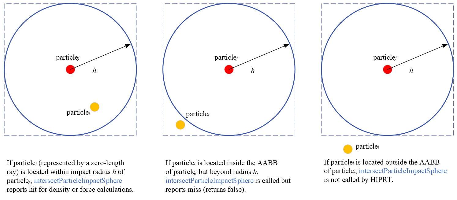
在 intersectParticleImpactSphere 中,我们获取射线起点作为粒子 的位置,以及粒子 的位置。然后,通过球形检查,剔除超出碰撞半径 的粒子。接着,我们利用 t(当前射线长度)和 normal 插槽,分别将平方距离 r2 和位移向量 d 的值存储到命中对象中,并将它们传递给主核函数程序。这些值将用于后续的密度和力计算。
对于第二次模拟迭代,我们有一个类似的核函数程序用于力评估。
extern "C" __global__ void ForceKernel(  hiprtGeometry  geom,  float3*         accelerations,  const Particle* particles,  const float*  densities,  Simulation*     sim,  hiprtFuncTable  table ){  const unsigned int idx      = blockIdx.x * blockDim.x + threadIdx.x;  Particle           particle = particles[idx];  float              rho      = densities[idx];
  hiprtRay ray;  ray.origin    = particle.Pos;  ray.direction = { 0.0f, 0.0f, 1.0f };  ray.minT      = 0.0f;  ray.maxT      = 0.0f;
  float pressure = calculatePressure( rho, sim->m_restDensity, sim->m_pressureStiffness );
  hiprtGeomCustomTraversalAnyHit tr( geom, ray, hiprtTraversalHintDefault, sim, table );
  float3 force = make_float3( 0.0f );  while ( tr.getCurrentState() != hiprtTraversalStateFinished )  {    hiprtHit hit = tr.getNextHit();    if ( !hit.hasHit() ) continue;    if ( hit.primID == idx ) continue;
    Particle hitParticle = particles[hit.primID];    float   hitRho      = densities[hit.primID];
    float3 disp        = hit.normal;    float  r           = sqrtf( hit.t );    float  d           = sim->m_smoothRadius - r;    float  hitPressure = calculatePressure( hitRho, sim->m_restDensity, sim->m_pressureStiffness );
    force += calculateGradPressure( r, d, pressure, hitPressure, hitRho, disp, sim->m_pressureGradCoef );    force += calculateVelocityLaplace( d, particle.Velocity, hitParticle.Velocity, hitRho, sim->m_viscosityLaplaceCoef );  }
  accelerations[idx] = rho > 0.0f ? force / rho : make_float3( 0.0f );}
ForceKernel 用于评估粒子 由于内部力产生的加速度贡献,其代码模式与 DensityKernel 相同。在这里,为了避免冗余的数据访问和计算以优化性能,当 = 时,我们跳过了对粒子 命中的计算。此外,我们使用与密度核相同的自定义相交函数。另外,基于公式 (4-7) 计算压力、压力梯度和粘性项的函数实现如下。
__device__ float calculatePressure( float rho, float rho0, float pressureStiffness ){  // Implements this equation:  // Pressure = B * ((rho / rho_0)^3 - 1)  const float rhoRatio = rho / rho0;
  return pressureStiffness * max( rhoRatio * rhoRatio * rhoRatio - 1.0f, 0.0f );}
__device__ float3calculateGradPressure( float r, float d, float pressure, float pressure_j, float rho_j, float3 disp, float pressureGradCoef ){  float avgPressure = 0.5 * ( pressure + pressure_j );  // Implements this equation:  // W_spiky(r, h) = 15 / (pi * h^6) * (h - r)^3  // GRAD(W_spiky(r, h)) = -45 / (pi * h^6) * (h - r)^2  // pressureGradCoef = particleMass * -45.0f / (pi * h^6)
  return pressureGradCoef * avgPressure * d * d * disp / ( rho_j * r );}
__device__ float3calculateVelocityLaplace( float d, float3 velocity, float3 velocity_j, float rho_j, float viscosityLaplaceCoef ){  float3 velDisp = ( velocity_j - velocity );  // Implements this equation:  // W_viscosity(r, h) = 15 / (2 * pi * h^3) * (-r^3 / (2 * h^3) + r^2 / h^2 + h / (2 * r) - 1)  // LAPLACIAN(W_viscosity(r, h)) = 45 / (pi * h^6) * (h - r)  // viscosityLaplaceCoef = particleMass * viscosity * 45.0f / (pi * h^6)
  return viscosityLaplaceCoef * d * velDisp / rho_j;}
对于最后的模拟迭代,我们组合了一个积分核函数程序,用于计算每个粒子内部力和外部力的合力,并根据公式 (8) 更新加速度、速度、位置和 AABB。
extern "C" __global__ void IntegrationKernel(  Particle* particles, Aabb* particleAabbs, const float3* accelerations, const Simulation* sim, const PerFrame* perFrame ){  const unsigned int idx          = blockIdx.x * blockDim.x + threadIdx.x;  Particle           particle     = particles[idx];  float3             acceleration = accelerations[idx];
  // Apply the forces from the map walls  for ( u32 i = 0; i < 6; ++i )  {    float d       = dot( make_float4( particle.Pos, 1.0f ), sim->m_planes[i] );    acceleration += min( d, 0.0f ) * -sim->m_wallStiffness * make_float3( sim->m_planes[i] );  }
  // Apply gravity  acceleration      += perFrame->m_gravity;
  // Integrate  particle.Velocity += perFrame->m_timeStep * acceleration;  particle.Pos      += perFrame->m_timeStep * particle.Velocity;
  Aabb aabb;  aabb.m_min = particle.Pos - sim->m_smoothRadius;  aabb.m_max = particle.Pos + sim->m_smoothRadius;
  // Update  particles[idx]     = particle;  particleAabbs[idx] = aabb;}
基于上一次迭代计算出的内部力加速度值,我们部署了一个简单的边界条件模型,该模型根据墙面和刚度参数 m_wallStiffness 反映粒子从撞击墙面时的运动,并将反射累积作为加速度值的外部力贡献。此外,我们还需要添加重力贡献。利用这个合加速度,我们可以轻松地依次推导出新的速度、位置和 AABB 值。
基于主机的实现,使用 HIP RT。
首先,我们定义了两个结构体来表示缓冲区 Simulation 和 Particle,用于存储必要的输入参数和粒子数据。
struct Simulation{    float  m_smoothRadius;    float  m_pressureStiffness;    float  m_restDensity;    float  m_densityCoef;    float  m_pressureGradCoef;    float  m_viscosityLaplaceCoef;    float  m_wallStiffness;    u32    m_particleCount;    float4 m_planes[6];};
struct Particle{    float3 Pos;    float3 Velocity;};
我们为如下描述的场景填充了这两个缓冲区的初始数据。
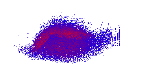
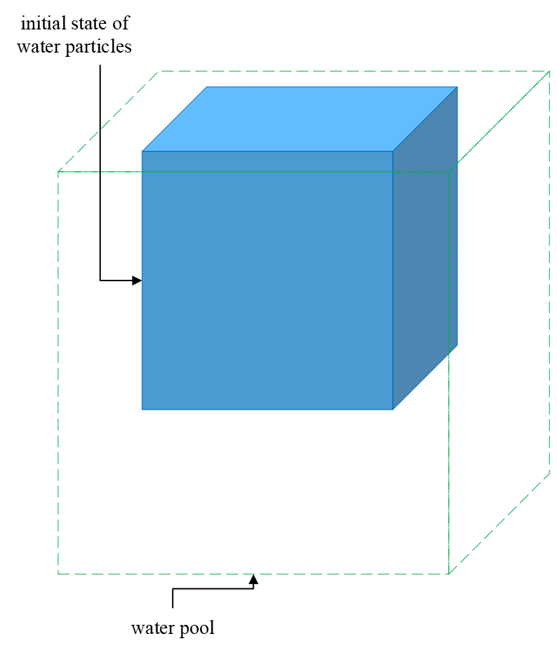
在一个 1 m³ 的立方形水池中,水粒子从水池顶部落下。水的初始体积为一个 0.216 m³ 的立方体。水粒子均匀分布在水体积中,粒子数量为 131,072。其他参数请参考水的属性,例如静止密度 1000 kg/m³,以及根据上述条件推导出的粒子质量。粘度值为 0.4。所有水池壁面的刚度值为 3000。粒子搜索半径指定为 0.02 m,即 SPH 平滑半径 。
接下来,射线追踪的一个非常重要的步骤是构建一个加速结构(AS)。在这里,为了方便起见,我们选择 hiprtGeometry,它只包含底层 AS。我们将 hiprtPrimitiveTypeAABBList 作为相应的 hiprtGeometryBuildInput 的类型。对于每个 AABB 元素,我们根据初始粒子位置填充初始数据。
hiprtAABBListPrimitive list;list.aabbCount = sim.m_particleCount;list.aabbStride = sizeof( Aabb );std::vector<Aabb> aabbs( sim.m_particleCount );for ( u32 i = 0; i < sim.m_particleCount; ++i ){ const hiprtFloat3& c = particles[i].Pos; aabbs[i].m_min.x = c.x - smoothRadius; aabbs[i].m_max.x = c.x + smoothRadius; aabbs[i].m_min.y = c.y - smoothRadius; aabbs[i].m_max.y = c.y + smoothRadius; aabbs[i].m_min.z = c.z - smoothRadius; aabbs[i].m_max.z = c.z + smoothRadius;}由于粒子 AABB 可以每帧更新,我们选择 hiprtBuildFlagBitPreferFastBuild 模式来构建加速结构,并将每帧重建整个 hiprtGeometry。
hiprtGeometryBuildInput geomInput;geomInput.type = hiprtPrimitiveTypeAABBList;geomInput.aabbList.primitive = list;geomInput.geomType = 0;
size_t geomTempSize;hiprtDevicePtr geomTemp;hiprtBuildOptions options;options.buildFlags = hiprtBuildFlagBitPreferFastBuild;CHECK_HIPRT( hiprtGetGeometryBuildTemporaryBufferSize( ctxt, geomInput, options, geomTempSize ) );CHECK_ORO( oroMalloc( reinterpret_cast<oroDeviceptr*>( &geomTemp ), geomTempSize ) );
hiprtGeometry geom;CHECK_HIPRT( hiprtCreateGeometry( ctxt, geomInput, options, geom ) );在这里,您可以看到 oro 函数,这些函数是 Orochi 库 的函数,该库封装了 HIP 和 CUDA API。因此,使用 Orochi 编写的代码也可以在非 AMD GPU 上运行。
然后,我们为自定义相交函数注册了函数表。如前所述,我们对密度核函数程序和力核函数程序都使用了相同的相交函数 intersectParticleImpactSphere。
hiprtFuncNameSet funcNameSet;funcNameSet.intersectFuncName              = "intersectParticleImpactSphere";std::vector<hiprtFuncNameSet> funcNameSets = { funcNameSet };
hiprtFuncDataSet funcDataSet;CHECK_ORO( oroMalloc(    reinterpret_cast<oroDeviceptr*>( &funcDataSet.intersectFuncData ),    sim.m_particleCount * sizeof( Particle ) ) );CHECK_ORO( oroMemcpyHtoD(    reinterpret_cast<oroDeviceptr>( funcDataSet.intersectFuncData ),    particles.data(),    sim.m_particleCount * sizeof( Particle ) ) );
hiprtFuncTable funcTable;CHECK_HIPRT( hiprtCreateFuncTable( ctxt, 1, 1, funcTable ) );CHECK_HIPRT( hiprtSetFuncTable( ctxt, funcTable, 0, 0, funcDataSet ) );
设置函数表后,我们可以相应地构建三个模拟迭代的核函数程序。同时,我们也分配了每个迭代的相应输出缓冲区。
// Densityfloat*      densities;oroFunction densityFunc;CHECK_ORO( oroMalloc( reinterpret_cast<oroDeviceptr*>( &densities ), sim.m_particleCount * sizeof( float ) ) );buildTraceKernelFromBitcode(    ctxt, "../common/TutorialKernels.h", "DensityKernel", densityFunc, nullptr, &funcNameSets, 1, 1 );
// ForcehiprtFloat3* accelerations;oroFunction  forceFunc;CHECK_ORO(    oroMalloc( reinterpret_cast<oroDeviceptr*>( &accelerations ), sim.m_particleCount * sizeof( hiprtFloat3 ) ) );buildTraceKernelFromBitcode(    ctxt, "../common/TutorialKernels.h", "ForceKernel", forceFunc, nullptr, &funcNameSets, 1, 1 );
// IntegrationPerFrame*  pPerFrame;oroFunction intFunc;{    PerFrame perFrame;    perFrame.m_timeStep = 1.0f / 320.0f;    perFrame.m_gravity  = { 0.0f, -9.8f, 0.0f };    CHECK_ORO( oroMalloc( reinterpret_cast<oroDeviceptr*>( &pPerFrame ), sizeof( PerFrame ) ) );    CHECK_ORO( oroMemcpyHtoD( reinterpret_cast<oroDeviceptr>( pPerFrame ), &perFrame, sizeof( PerFrame ) ) );    buildTraceKernelFromBitcode( ctxt, "../common/TutorialKernels.h", "IntegrationKernel", intFunc );}
最后,我们可以构建一个主模拟循环来按顺序分派 HIP RT 核函数。对于每一帧的迭代,我们首先重建 HIP RT 几何以更新 AS,然后启动核函数程序,并将所需缓冲区的指针放入核函数的入口参数中。
const u32 b   = 64; // Thread block sizeu32       nb = ( sim.m_particleCount + b - 1 ) / b; // Number of blocks
// ...
// Simulatefor ( u32 i = 0; i < FrameCount; ++i ){    CHECK_HIPRT( hiprtBuildGeometry( ctxt, hiprtBuildOperationBuild, geomInput, options, geomTemp, 0, geom ) );
    void* dArgs[] = { &geom, &densities, &funcDataSet.intersectFuncData, &pSim, &funcTable };    CHECK_ORO( oroModuleLaunchKernel( densityFunc, nb, 1, 1, b, 1, 1, 0, 0, dArgs, 0 ) );
    void* fArgs[] = { &geom, &accelerations, &funcDataSet.intersectFuncData, &densities, &pSim, &funcTable };    CHECK_ORO( oroModuleLaunchKernel( forceFunc, nb, 1, 1, b, 1, 1, 0, 0, fArgs, 0 ) );
    void* iArgs[] = { &funcDataSet.intersectFuncData, &list.aabbs, &accelerations, &pSim, &pPerFrame };    CHECK_ORO( oroModuleLaunchKernel( intFunc, nb, 1, 1, b, 1, 1, 0, 0, iArgs, 0 ) );
    // ...}
结论
HIP RT 具有与 DXR 和 Vulkan RT 类似的功能,它提供了一种更简单、更灵活的替代方案来实现流体模拟中使用的点查询进行邻域搜索,方法是利用快速动态几何体加速结构更新和自定义相交函数。邻域搜索的 BVH 遍历可以由 HIP RT 高效地自动隐式完成。我们最近发布了新版本的 HIP RT (v.2.1),其中添加了更多功能。我们很乐意听取您关于 HIP RT 的有趣用例。
此示例已包含在 HIP RT SDK 教程中 (https://github.com/GPUOpen-LibrariesAndSDKs/HIPRTSDK)。
- 核函数程序的代码:https://github.com/GPUOpen-LibrariesAndSDKs/HIPRTSDK/blob/main/tutorials/common/TutorialKernels.h
- 主机端 C++ 代码:https://github.com/GPUOpen-LibrariesAndSDKs/HIPRTSDK/blob/main/tutorials/14_fluid_simulation/main.cpp
- 一些相关数据结构定义:https://github.com/GPUOpen-LibrariesAndSDKs/HIPRTSDK/blob/main/tutorials/common/FluidSimulation.h
参考文献
- R. A. Gingold, J. J. Monaghan, Smoothed particle hydrodynamics: theory and application to non-spherical stars, Monthly Notices of the Royal Astronomical Society, Volume 181, Issue 3, December 1977, Pages 375–389, https://doi.org/10.1093/mnras/181.3.375
- Takahiro Harada; Seiichi Koshizuka; Yoichiro Kawaguchi (2007). Smoothed particle hydrodynamics on GPUs. Computer Graphics International. pp. 63–70。
- Tianchen Xu; Wen Wu; Enhua Wu (2014). Real-time generation of smoothed-particle hydrodynamics-based special effects in character animation. Computer Animations and Virtual Worlds, 25: 185–198。
- DirectX Raytracing (DXR) Functional Spec, https://msdocs.cn/DirectX-Specs/d3d/Raytracing.html
- Vulkan 1.3 specification, https://registry.khronos.org/vulkan/specs/1.3/html/
- Matthias Müller, David Charypar, and Markus Gross. 2003. Particle-based fluid simulation for interactive applications. In Proceedings of the 2003 ACM SIGGRAPH/Eurographics symposium on Computer animation (SCA ‘03). Eurographics Association, Goslar, DEU, 154–159, https://matthias-research.github.io/pages/publications/sca03.pdf